Mathematical modelling of the gravitropic reaction in fungi and plants
We have done a great deal of research on gravitropism in mushrooms, during which we collected an enormous quantity of detailed measurements of the process in live mushrooms. Looking at the amount of data we had accumulated we began to think in the mid-1990s that we might have enough data to create a mathematical model of the gravitropic reaction in fungi.
This page describes several mathematical models of the gravitropic reaction that were created by the late Alvydas Stočkus [Dr. Alvydas Stočkus was killed in an accident in February 1996] and Audrius Meškauskas (both of whom were trained in biomathematics at the Institute of Botany, Lithuania), in co-operation with David Moore in the School of Biological Sciences at The University of Manchester, United Kingdom.
Our main research area at the time was mathematical modelling of the spatial organisation of the gravitropic reaction in stems of the small ink-cap mushroom Coprinopsis cinerea. This work belongs to the historical period of bioinformatics, when genome sequences were not yet available, and some scientists tried to use bioinformatical methods for analysis of other very large data sets obtained from a variety of experiments.
GravitropismMany plant organs grow strictly upwards (for example, shoots) or downwards (for example, roots). Mushroom fruit bodies also try to keep a strictly vertical orientation, because this is essential for their spore distribution. Mushroom spores simply fall from the gills into turbulent air currents beneath the cap; so they depend on exact verticality of the gills to avoid falling from one gill to only land on the neighbouring gill surface. When such organs are turned away from the vertical by some angle, they start to bend toward the vertical position. This reorientation in the gravity field to maintain a specific position is defined as gravitropism. Some organs grow neither strictly up or down, but at a particular angle from the vertical. This phenomenon is called plagiogravitropism, and it accounts for (among other things) tree branches growing horizontally, or the branches of bushy plants growing at 40-45° from the vertical. |
The gravitropic response is a very complex phenomenon, and two general strategies can be adopted in creating mathematical models. In one approach the specific characteristic of particular parts of the biological system are used as modelling parameters in attempts to produce a realistic simulation of the biological process. The alternative approach differs in that the basis of the model is independent of the real processes; rather, it is dependent on the informational content of those processes for an organism. These imitational models use abstract terms such as 'physiological signal' rather than exact parameters like 'substance concentration'.
The advantage of such approaches is that they can mimic or simulate the overall picture of events in gravitropically responding organs without requiring detail about how the tropic response is realised in life. The resultant model can be an abstraction, which can be applied to a wide range of subjects. Indeed, the model groups described on this page were successfully used in simulating and predicting tropic responses in such different groups as fungi and plants.
Comparison of the behaviour, predicted by a certain model, with actual experimental data can be used to explore the processes further, even taking the analysis into conditions that are currently not possible or very difficult to measure directly. Also, when the model identifies critical features, experimental application of specific inhibitors sometimes make it possible to establish closer relations between abstract model parameters and actual components of the biological system.
As a rule, the models created in this way are predictive. For example, having been fitted into the gravitropic reaction of an object under the Earth-standard 1× g gravitational acceleration, they have the potential ability to predict how the gravitropic process would develop under 2× or 0.5× g. The models can also be used to simulate the gravitropic bending from different initial angles of disorientation. In suitable programs the user is able to change such environmental parameters easily and then see the behaviour predicted by the model. The ability to make correct predictions under changed conditions can be a serious criterion when it is necessary to choose between alternative hypotheses.
Examples of alternative hypothesesMany plant organs (for example, oat coleoptiles) bend after reorientation into the horizontal position, but stop bending before reaching the vertical position. It is possible to write a mathematical model where this termination is determined by a plagiogravitropic component. However, the plagiogravitropism would direct bending from the vertical (towards the 'preferred' angle of the plagiogravitropic reaction. If such bending is not observed experimentally (as a rule, coleoptiles don't bend from vertical position), some alternative model might be more credible. Similarly, the apical part of the gravitropically bending organ sometimes starts to straighten before the apex reaches the vertical position (the critical angle is about 35 angular degrees in mushroom stems of Coprinopsis cinerea). It is possible to explain this by supposing that the apical part is plagiogravitropic at this angle. However, such a model would wrongly predict the bending of the apex away from the vertical position toward this supposed angle. Hence, much more complicated explanations of the phenomenon of straightening must be taken into consideration. The straightening reaction, mentioned above, need not be made part of a working model providing attention is restricted to the apex angle. However, if we compare the whole shape of the bending organ with the experimental data, the successful model can only be written if we suppose that gravitropic bending is complemented by some curvature compensation (that is, a straightening) reaction. The exact mechanism of this reaction is still not clear, hence this is the area where the advantages of the more abstract imitational models can be successfully used. Evidently, several alternative models can sometimes be successfully fitted into one set of experimental data. However, as a rule, it is possible to choose between them using wider knowledge about the object being explored. |
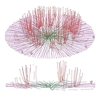
Our modelling exercises developed out of an extensive series of experimental observations on the spatial organisation of gravitropic curvature in stems of the small ink cap mushroom Coprinopsis cinerea. The gravitropic bending of base- and apex-pinned Coprinopsis cinerea stems was recorded on videotapes. The images were captured from the tapes after each 10 min, and transformed by image analysis software into tables of changing co-ordinates of points for each stem. The non-linear regression of these points was performed using Legendre polynomials. From the resulting equations the patterns of changing local curvature for 50 subsections of each stem during 400 min of gravitropic reaction were calculated (and this was done for a great many stems).
All of these observations were published in the scientific literature. A note about the data most relevant to mathematical modelling is included on the accompanying page [CLICK HERE to open in a new window][OR fetch a PDF version], and most of the publications are made available on the page entitled Neighbour-Sensing documentation [CLICK HERE to open in a new window][OR fetch a PDF version].
So far we have created two types of model:
- The earliest models, developed by the late Alvydas Stočkus (and applied to fungi in collaboration with David Moore), were imitational models designed to imitate specifically the change of the angle of the stem apex during the gravitropic reaction. The output is a graphical curve, indicating how the apex angle changes with time. The models were successfully used to imitate the gravitropic reaction of various subjects from the plant and fungal kingdoms. Information on how the apex angle changes with time is often the only information available in the reference (observational) data for your object of interest. Hence, despite the availability of our later models on spatial organisation of the gravitropic reaction, it can still be useful to use the apex-angle based model. For more detailed description and discussion of this and related models see Stočkus (1994) and Stočkus & Moore (1996) in our list of publications.
- The most recent model, developed by Audrius Meškauskas and David Moore, are models that simulate the complete spatial organisation of the gravitropic reaction. The output is a set of calculated representations (hypothetical images) of the bending organ, indicating how the whole shape changes with time. Hence the output of this model can be much more strictly compared with experimental data, providing the possibility of reaching more exact conclusions.
Imitational models developed by the late Alvydas Stočkus
Description of the apex angle-based models of the gravitropic reaction without the maths
The difference in growth rates between opposite flanks of an axial organ is the cause of gravitropic curvature. In fact, such a specific definition is not necessary for imitational modelling. For modelling purposes, it is usually enough to assume that curvature just occurs in response to some signal. The factor (or factors) which code the delivery and intensity of this curvature in the modelling were considered to be the 'physiological signals' for tropic bending.
Essentially, this group of models assume only one gravitropic signal, which is generated in the perception stage and then carried to the site of its realisation, where it is used to cause the growth differential.
For strictly positively or negatively gravitropic organs (such as mushroom fungus fruit body stems) the physiological signal at the stage of perception is proportional to the sine of the angle between the apex and the true vertical.
If the organ then grows to another specific angle (from the horizontal), this signal is proportional to the sine of the difference between the initial apex angle and the subsequent apex angle.
During the transmission of the signal the usual paths for transduction of physiological signals are used (that is, no special constraints are imposed by the model). The time, required for transduction of the signal is the main reason for any time delay between the onset of gravitropic stimulation and the start of tropic bending.
However, this time interval may also include those time delays required for signal perception and realisation as well, because, at the present stage of modelling, these times are not separable. Hence, the signal level at the realisation site is proportional to the signal level in the apex as it was a certain (unknown or notional) time before.
During the realisation of the gravitropic response, the bending acceleration (not speed) is proportional to the difference of two factors. The first factor is the level of the gravitropic signal in the realisation site. The level of the second factor is proportional to the bending speed. It may be related to some internal system(s) for regulation of the gravitropic response.
This model can be successfully fitted to the gravitropic reaction of many objects from both plant and fungal kingdoms. More information about this and other apex-angle based models, created in our research, can be found in our list of publications.
Mathematical description of the apex angle-based model of the gravitropic reaction
Most gravitropism experiments start with the experimenter reorienting a normally-growing plant or fungal organ; and indeed, in most cases the reorientation is specifically from the vertical to the horizontal. This modelling is based on the assumption that after reorientation the physiological signal arises in the apex (this is the signal perception) and that this signal at any time t is proportional to the cosine of the tip angle at this time:
(1) |
Where the tip angle is measured as the angle from the horizontal. To simulate the gravitropic reaction under different gravitational accelerations, Ks can be replaced by Ks g , where g is the gravity vector in relative units (1.0 on the Earth). It is possible to combine ideas about plagiogravitropisms into this equation by writing the perception function as:
(1a) |
Here, beta (β) is the angle of gravitropic reaction (90 degrees for strictly positive or negative gravitropism, lower values for plagiogravitropism). This function can also be written in alternative, but mathematically identical ways, for example as the sum of sine and cosine.
After perception, the signal is transmitted in the basipetal direction. In this model, the classic equation of signal transmission was used:
(2) |
This equation means that signal in the realisation site, S is equal to the signal level in the apex as it was time τ (tau) before. NOTE that this model simplifies the bending process to a rotation around one joint, there is no attempt to simulate the natural bending process.
During realisation of the gravitropic response, the bending acceleration (not speed),
 |
is proportional to the difference of two factors. The first factor is the level of gravitropic signal at the realisation site, S. The level of the second factor is proportional to the bending speed. It may be related to some internal systems concerned with regulation of the gravitropic response.
Hence,
 |
(3) |
By joining together the equations mentioned above, we obtain the final equation:
 |
(4) |
This is a second order differential equation with delay. It can be solved easily using classic numerical methods of solution. To underline the biological meaning of the components (first perception, then the signal delay) it can be rewritten as:
 |
(4a) |
This mathematical model, which was created by the late Alvydas Stočkus, was realised as a JavaTM simulation program by Audrius Meškauskas. The Java simulation predicts how the apex angle changes during the process of the gravitropic reaction in the mushroom fruit body stem of the small ink cap mushroom Coprinopsis cinerea, and plots the appropriate apex angle versus time graph. At the user's discretion, real experimental observations can be plotted as well.
The program allows the user to modify external factors such as the strength of the gravity vector and the initial angle of orientation, so it will predict the exact results of so far untried experiments on the values of these factors. It is thereby open to experimental verification. You might like to find out, for example, how a fruit body would react to being placed horizontal on the surface of Mars (g = 0.38), Saturn (g = 0.92) or Jupiter (g = 2.36). The model will predict how the Coprinopsis stem will respond in each of these circumstances. We leave it to you to arrange how to test those predictions, but when you do, you can add your own experimental data to the built-in data sets to compare your experimental results with the predictions of the model. Bon voyage! Do wrap up well, Mars can be chilly this time of year.
Models simulating spatial organisation of the gravitropic reaction developed by Audrius Meškauskas
Description of the spatial organisation model of the gravitropic reaction without the maths
The difference of growth rates between opposite flanks of an axial organ is the cause of the gravitropic curvature that generates the changing apex angle; but this model concentrates on the morphogenesis of the curvature, effectively relegating the apex angle to a side-effect of those morphogenetic events.
Again, the underlying basic scheme of the model can be traced back to Rawitscher (1932) and Merkys et al. (1972) as described in the Information Box above. The model assumes that during the gravitropic reaction the bending process is determined by the following factors (or signals):
- Gravitropic signal, perceived in the apex and transmitted to the bending subsection (which is the realisation site).
- Gravitropic signal, perceived in the bending subsection.
- Curvature compensation, or straightening, signal, perceived in the realisation site. This signal is proportional to the local curvature of the bending subsection. This signal was introduced to explain the straightening of the apical part before it reached the vertical position.
The local bending speed in the subsection is determined by the sum of these three signals. The gravitropic signals are positive, causing bending. The curvature compensation signal is negative. Such integration of signals in the hypothesis allows us to create a mathematical model, which is able to reproduce the real spatial organisation of the gravitropic reaction in the stem of the mushroom Coprinopsis cinerea.
Mathematical description of the model of spatial organisation of the gravitropic reaction
The basic scheme of the model started from the same premise as described above, that after reorientation the physiological signal arises in the apex (signal perception), and that this signal at any time t is proportional to the cosine of the tip angle at this time:
(1) |
After perception the signal is transmitted in a basipetal direction. We established that the 'wave with decrement', which is most commonly used to describe signal transmission, cannot alone explain the development of curvature in a mushroom stem. The main argument is that the point of bending of a mushroom stem (Coprinopsis cinerea in our experiments) moves in a basipetal direction with decreasing speed, which is not characteristic for the 'wave with decrement' equation. However, if an autotropism in the realisation point is also included, the combination explains this phenomenon. Hence, in this model, the classic equation of signal transmission was used:
(5) |
where λ is the relative distance from the base of the axial organ (0 = base, 1 = tip), and v is the signal transmission speed, which is constant for a wave equation. Hence the signal reaches the certain realisation point delayed by time (1-λ)/v and the signal level exponentially decreases during transmission (constant SDE determines this decrement).
If we now suppose that the local bending velocity is simply proportional to this local signal level S(λ,t), we obtain a model very similar to the equation (4) above. However, for exact simulation of the spatial development of the gravitropic reaction in Coprinopsis cinerea the description of the realisation must be a more complicated function, which is not only derived from S(λ,t), but also involves two additional signals: the curvature compensation (or straightening) signal and a local perception function.
The compensation signal arises at the same point where the bending process develops; that means it is not transmitted through the stem. This signal was introduced to explain the straightening of the apical part of the living stem before it is restored to the vertical. The level of this signal was assumed to be proportional to local curvature, CL (see explanations in the Information Box below; OR fetch a PDF version).
The curvature compensation reactionCheck out the accompanying page for:
CLICK HERE to open the page in a new window [OR fetch a PDF version] |
It is known that the compensation process is much more strongly expressed closer to the apex than in lower (but still apical) subsections. To produce the working model, it was necessary to take this fact into account. Hence, it was assumed that the distribution of ability for the straightening reaction is not uniform and exponentially decreases in the basipetal direction.
The level of the straightening signal at position λ at any given time t is:
(6) |
here parameters AU and AD determine the distribution of autotropism along the stem.
The proposition that perception of the gravitropic signal takes place in the stem apex is enough to create the mathematical model that can reproduce all stem shapes observed to occur in Coprinopsis cinerea during the gravitropic reaction of live stems.
However, it can’t simulate the process as it develops in time (goodness of fit tests indicate significant differences between model-predicted and observed shapes). The bending process, simulated by this simple model, is too slow in the beginning of the gravitropic reaction (in approximately the first three hours) and too fast in the later stages.
Hence, we included the local perception of the signal as a parameter; a feature which is confirmed both experimentally (Greening, Holden & Moore, 1993) and by mathematical modelling (Meškauskas, Moore & Novak Frazer, 1998).
It was assumed, that the hyphal system has a level of autonomy sufficient not only to respond to the signal from the tip, but also to perceive the gravitropic 'irritation' in the site of realisation. After adding this parameter, we achieved exact simulations. However, it was necessary to assume that the local perception function [explained and illustrated on this page] differs significantly from the perception function in the apex and can be approximated as
(7) |
Similarly to sin(αL), this function is maximal when αL= zero (horizontal position) , but it can reduce much faster when the parameter αL starts to increase. Hence it was supposed that local perception plays the most important role in the initial stages of the bending process, when the αL is less than 45 degrees.
The essential condition to satisfy goodness of fit tests was also to assume that the distribution of ability for local perception [explained on this page] is not uniform, but exponentially decreases from the apex in the basipetal direction. Hence the level of the local perception at the time t in the position λ is:
(8) |
Hence, the realisation of the gravitropic response, the local bending speed in point λ at time t is:
(9) |
where KW is the realisation constant. By summarising the equations shown above and expressing local angle through local curvature, we obtain the final equation (equation 10) below:
(t>0; 0 <= λ <= 1, initial condition CL( λ,0) =0 (straight stem); boundary conditions CL(t,0) = CL(t, λ)=0) Equation 10 |
Using this equation, the program was written in Java to obtain numeric solutions.
The mathematical models presented in these web pages, and some of the background research, are described in much more detail in the publications detailed on the page entitled Neighbour-Sensing documentation [CLICK HERE to open in a new window][OR fetch a PDF version].
Copyright © David Moore, A. Meškauskas & L. Novak-Frazer 2017