Overview of the Neighbour-Sensing model without the maths
The program simulates growth of fungal mycelia in three-dimensional space. The mycelium is currently represented as a tree-like structure. All ends of this tree are the cyberhyphal tips and they can branch, grow, and alter their growth direction in response to different tropisms to which the user makes them reactive.
The process of simulation is performed by a loop algorithm for each currently existing hyphal tip of the mycelium. Each time the loop is performed (that is, at each ‘iteration’) the algorithm does this:
- it finds the number of neighbouring segments of mycelium (N). A segment is counted as neighbouring if it is closer than the given critical distance (R). In the simplest case, we did not use the concept of the density field, preferring a more general formulation about the number of the neighbouring tips.
- if N is less than the user-specified number of neighbours required to suppress branching (that is if N<Nbranch), there is a certain given probability (Pbranch) that the tip will branch. If the generated random number (0..1) is less than this probability, the new branch is created and the branching angle takes a random value.
Randomised branch generation was similar overall to earlier models in which distance between branches and branching angles followed experimentally measured statistical distributions. This, however, was not required to achieve realistic colony shapes in our model, and we used a uniform randomised distribution. We assumed that all hyphal tips in mycelia grow at constant speed. This assumption was sufficient to achieve realistic shape and structure of the colony.
In this mathematical model the growth vector of each virtual hyphal tip, at each iteration of the algorithm, depends upon values derived from its surrounding virtual mycelium. The growth vector is being informed of its surroundings so, effectively, the virtual hyphal tip is sensing the neighbouring mycelium. This is why we call it the Neighbour-Sensing model.
Following the lead of previous workers, we assumed that abrupt change of the growth direction of hyphae are generally unlikely, so we made the tip change direction gradually. This is achieved by implementing a “persistence factor” so that growth direction changes gradually, during several iterations of the algorithm. In our implementation, the growth speed remained constant and the density gradient alters only the growth direction. Otherwise, a high gradient, if formed accidentally, would cause unrealistically fast growth in some parts of the mycelium.
With low values of the persistence factor the model is able to form small linear structures. This is because, with such a parameter set, immediately after branching the hyphal density field tends to orient the new tip strictly in the opposite growth direction from the old tip. That is, the new hypha is directed to grow parallel with the old hypha but in the opposite direction. If we suppose that the hyphal density field is generated just by tips and branch points, this direction remains optimal until the tip goes sufficiently far from the branch point to start interacting with other hyphae. Changing parameters while the colony is still nearly linear can produce ellipsoidal or tubular cybermycelia.
The model implements two mechanisms to regulate branching. In one mode, the neighbouring hyphal tips and/or branch points are counted, and branching is allowed if their number is below a threshold value (which is set by the experimenter). In the alternative mode, branching is allowed if the hyphal density field, used for the tropic reaction (see below) is lower than a threshold value (again set by the experimenter).
In both cases, it is additionally assumed that if branching is possible, there is only a certain probability that it will happen during the current iteration. The initial direction of any branch that is formed may be randomized or may immediately be oriented by tropic reactions; the experimenter determines which of these operates.
Tropisms were implemented using the concept of a density field, it being supposed in the model that each point of the mycelium contributes to a field that can be described by the formulas used to describe electric and gravitational fields in physics (because these are well understood). The program implements positive and negative autotropic reactions by orienting the growing hyphal tip towards (= positive) or against (= negative) the gradient of this field. The impact of the short range autotropic reaction is inversely proportional to the square of the distance to the point generating the hyphal density field.
To obtain more diverse structures (we are interested in the form and construction of fungal fruit bodies), we also implemented a long range autotropic reaction. The long range autotropic reaction is made directly proportional to the square root of distance. The direct proportionality (the larger the distance, the stronger the interaction) can be realistic if it is assumed that it depends on a mechanism by which the 'attractant' is released in an inactive form and slowly changes into active form while it diffuses.
One of our hopes was to be able to produce polarized structures. Such structures can be easily generated by supposing an additional orientation field. This is a directed field, and the hyphal tip can be set to orient itself to any angle (as set by the experimenter) in relation to the vector of this field. A realistic analogy of this orientation field could be the gravitational field; in which case the orientation angle sought by the hyphal tip would be called a diagravitropism. This orientation incorporates a tolerance angle to prevent the tip hunting around the optimum.
The model space can contain multiple additional objects (we call them “substrates” although they can also be given the characteristics of growth inhibitors) that generate their own field, causing positive or negative tropisms for the growing hyphal tips. The size, position and other parameters of such substrates can be set interactively and, if required, altered at later stages during the simulation.
All parameters are adjustable and can be altered before the start of growth, or the growth process can be paused and the parameters changed during the simulation. The interactive (Java) environment allows the generated three dimensional mycelia to be viewed in any orientation, saved as images and/or saved as data.
We have experimented with a variety of extensions of the model (we’ll give you hyperlinks to our publications later): for example, growth being suppressed by a high number of neighbouring tips; or allowing the growing tip only to be active for a fixed time before it stops growing and branching. Such changes can result in more optimal packing of the hyphae, but are not required to form a spherical colony.
Real fungal colonies are rarely uniform in structure, so the question arises whether any smaller new structures can form in a virtual colony growing in accordance with this model. We found that this could happen following abrupt changes of the model parameter set (especially R and Nbranch).
To enable viewing of the internal structure of the mycelia, the system can display slices of the object. Slice plane, slice thickness and slice orientation can be varied interactively.
Obviously, the computation load increases with increase in the number of hyphal tips the model creates. However, even when we started, the basic model was within the scope of desktop computers of the day (a 2.7 GHz Pentium machine could “grow” a mycelium of 5000 hyphal tips in about 45 minutes).
For larger structures like fungal fruit bodies single-processor computers of the day were not adequate and we ran the program on a supercomputer, utilising several processors in parallel mode.
This was one reason for implementing the model in Java as this allowed the same program to be run on different computer types.
Java is a general-purpose computer programming language specifically designed to allow application developers to 'write once, run anywhere' (WORA), meaning that compiled Java code can run on all platforms that support Java without the need to be recompiled. Java applications are typically compiled to bytecode that can run on any Java virtual machine (JVM) regardless of computer architecture. Java is an object-oriented language similar to C++, but simplified to eliminate language features that cause common programming errors. Java source code files (files with a .java extension) are compiled into bytecode files with a .class extension, which can then be executed by a Java interpreter. [source: https://en.wikipedia.org/wiki/Java_(programming_language] [and see JAVA+YOU at java.com CLICK HERE to open this website in a new window]. |
Today’s multi-processor PCs, tablets and even phones mean that processing power is no longer an issue. Unfortunately, the security issues that surround Java have made an issue of our model’s dependence on Java applets, because the digital security certificates needed for such applets to run '...on any Java virtual machine...' have proved to be impossible for individual programmers (like us) to obtain.
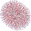
Nevertheless we have found a way to make the programs available over the Internet (view the Downloads Page) but before you go that far, we can show you a video of the program in operation. In order to allow maximum screen space to the simulation, it is started in a window that is empty except for controls around the frame and the one starting hyphal tip, which should be in the centre of the window.
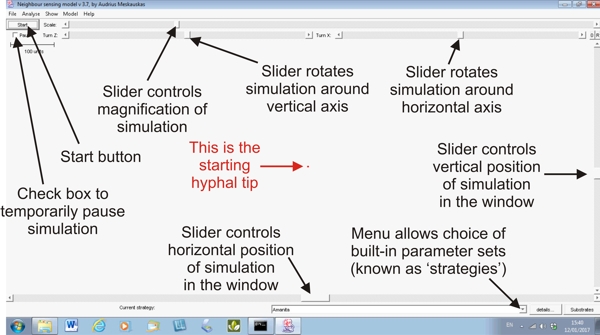
Think of the starting hyphal tip as a spore waiting to germinate. It exists in a large three-dimensional data space, and the on-screen view is literally a window onto this data space. Your view of that data space can be moved up and down with a slider control on the right frame, and from side to side with a slider control on the bottom frame; and, along the top frame, there is a slider that zooms your view, and so controls the magnification of the simulation under observation.
The simulation is started using a start button in the top left corner of the frame, and immediately beneath that start button is a pause switch in the form of a check-button. Click on that to temporarily pause the simulation (so you can inspect it, maybe change the view, or even change the parameters) and then click on the pause check-button again to resume the simulation. A view of the Neighbour-Sensing modelling window is shown below, with some of its main features labelled.
 |
From the panel below you can download a short (it runs for just under two minutes) video showing a Neighbour-Sensing simulation being produced. The same video is offered in a number of formats; choose the one which is appropriate to your device and software.
The legend in the panel below describes what's going on in the video and emphasises the points of interest that you should notice.
Sample video Cyberfungus02.wmv this is a WMV file (Windows Media Video) first introduced by Microsoft in 1999Sample video Cyberfungus02.mp4 this is an MP4 (or MPEG-4) file, a format first released in 2001 and currently accepted by computers, tablets, phones, game consoles, TVs and other devices manufactured by Apple, Microsoft, Samsung, HTC, Google, Huawei, Amazon, Lenovo and other brands; besides being widely accepted by media players and video software across the Internet.Sample video Cyberfungus02.mov this is a MOV file, introduced by Apple in 1998, an MPEG-4 format used in Apple's Quicktime program. MOV files use Apple's proprietary compression algorithm.Sample video Cyberfungus02.avi this is an AVI file (Audio Video Interleaved) introduced by Microsoft in November 1992Sample video Cyberfungus02.swf this is a SWF (Small Web Format) Adobe Flash file format for the Adobe Flash Player
|
Run VT!Well, I suppose the number of people likely to remember Roland Rat on morning TV in the early 1980s is fast declining, so what I mean is: play the video ... When you DO play the video you will see the blank screen shown in the panel immediately above (without the labels!). The first activity is to choose a 'strategy' or parameter set from the menu of built-in sets (we indicate how parameter sets are put together on Liam McNulty's page below). The menu offers Boletus, Amanita, Trichoderma, Random, Conus (which makes a conical mycelium), Cords (which makes strands of parallel hyphae), and standard (a 'general purpose' starting set). I choose the Amanita strategy and immediately press the Start button. You can see that the simulation has started by the appearance of descriptive numerals in the bottom left corner of the frame [for example: time 8 (8 program time units have elapsed), tips 3 (the mycelium has produced three hyphal tips), length 12.7 (total length of hyphae produced = 12.7 program length units), and unit 4.23 (average length of each hyphal segment)]. Mais quel dommage! We can't see the simulation on screen because I failed to centre the starting hyphal tip in the field of view before pressing the start button!! Cue panic as I scramble to adjust the right hand slider to bring the simulation down to the field of view, and then the slider on the bottom frame to set it into the centre. Note, though, that while this adjustment is being done the simulation continues serenely. This is generally true of the orientation controls (field of view, rotation, magnification) they operate while the simulation proceeds. The simulation is then allowed to continue to 132 time units (= 136 tips), at which time I click the pause check box to stop the simulation. I then activate the rotation controls at the top of the frame. Rotating the mycelium first around the horizontal axis and then around the vertical axis (notice that the amount of rotation is shown in angular degrees just to the left of each slider), in order to inspect the three dimensionality of the mycelium. That done, I click the small button labelled 0 (zero) at top right and this sets the rotations back to zero degrees. Then I move my attention to the magnification (scale) of the simulation by moving the scale slider at the top of the frame. Note how the scale bar (top left of the field of view) expands as this is done. Note also that this control does not affect the simulated mycelium. This is, effectively, a zoom control, which allows you to zoom into the mycelium to inspect closely the cyberhyphae and their branching system. Pause the final stage of the video for a while to appreciate some of the detail the most magnified stage reveals:
|
That should have given you a feel for the way the program works. In the next few pages we'll give you the underlying detail about how it works, and show how it can be used experimentally.
Read on!
Copyright © David Moore 2017