
2.3 Describing the evolution of biomass
In many instances, models such as those described on the previous page are applied to descibing the evolution of biomass by converting the total mycelial length to a weight of biomass. This is particularly useful when the fungus is grown in an industrial or biotechnological context. This area of research has therefore attracted much attention and some of the other attempts to model biomass evolution are now discussed.
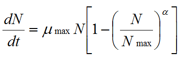
When grown on solid media, mycelial colonies are limited by space and by nutrient supply. Thus their exponential phase of growth is finite in length, and biomass evolution can be compared to the growth of populations modelled using the logistic equation:
where α is any real number, N is the number of individuals and μ, the specific growth rate |
(3) |
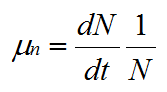
The specific growth rate, μ, is defined as:
 |
(4) |
and μ decreases as a negative linear function of population size according to:
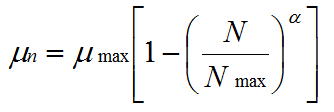 |
The curves generated by these equations are similar to the (sigmoidal) experimental curves of biomass evolution in batch cultures of filamentous fungi, where N would be replaced by the biomass, X.
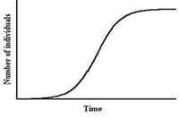 |
| Fig. 1. A typical curve generated by the logistic equation. As shown, the y-axis = number of individuals (N), but biomass (X) can replace N on the y-axis. |
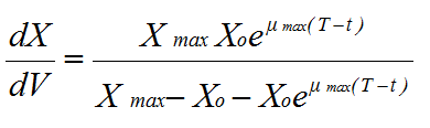
Koch (1975) modified the logistic equation so that it could be applied directly to mycelial growth by replacing N with the change in biomass with respect to volume, and changing the time variable to (T - t), where T is the time since the mycelium began growing, and t is the time when growth entered the unit volume under consideration. Thus the equation was rewritten, when integrated with respect to t, as:
where X0 is the initial biomass |
(6) |
Equation (6) was further modified to describe the increase in biomass when the colony radius extended linearly. However, this modification makes two contentious assumptions: (a) it assumes that the colony is a regular, flat disc (which is unrealistic); (b) it relies on the relationship between radial extension rate and specific growth rate, which assumes that the peripheral growth zone, ω, is constant in the equation:
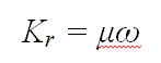 |
(7) |
However, this parameter varies from species to species and under different environmental conditions, so the modified equation is effectively limited to regular disc-shaped colonies growing on uniform media.
In order to be predictive (as opposed to descriptive), a model must contain a microscopic parameter that accurately represents a biological parameter, and which can be changed to test how it affects overall growth and development.
Viniegra-Gonzalez et al. (1993) developed the first model able to do this. It modelled the microscopic development of the mycelium based on the mathematics of symmetric binary trees. This was then used in a macroscopic description of the overall evolution of biomass, based on the logistic equation, that accounts for the proportion of inactive biomass (equivalent to the proportion of dead hyphae) in the mycelium by varying the coefficient α in equation (3).
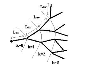 |
| Fig. 2. A schematic of a symmetric binary hyphal tree growing at a mean extension rate (from Viniegra-Gonzalez et al. 1993) |
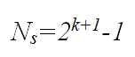
The microscopic component of the model redefined simple growth kinetic laws in terms of a branching level parameter, k. In a symmetric binary tree (illustrated above) every branching level is associated with a number of tips, Nt, according to the equation:
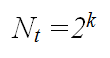 |
(8) |
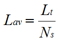
The number of segments, each of average length Lav, can also be calculated:
|
(9) |
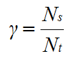
If:
 |
(10) |
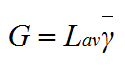
and
 |
(11) |
Then equation (2) can be rewritten as:
 |
(12) |
If a hypha branches at a critical biomass, Xc, the total biomass can be obtained from:
 |
(13) |
A time element can be introduced by the expression (see Fig. 2):
 |
(14) |
Calculating μx according to equation (7) having substituted in equations (12), (13) and (14), and recalling that dX/dt=dX/dy.dy/dt and d(2y)/dt = Ln2.2y(dy/dt); where y = bar-k+1, dy/dt= Ē /Lav, we then obtain:
 |
(15) |
This expression allows the calculation of μx when the only parameter measured is the number of tips (provided the value of Xc is known).
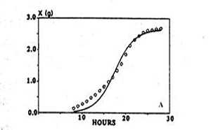
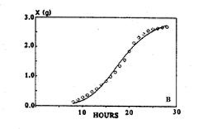
When reformulated in terms of X to describe macroscopic growth, statistical analysis showed that the equation described the evolution of biomass of Aspergillus niger more closely than the logistic equation (Fig. 3). Thus, macroscopic growth had been modelled with microscopic parameters.
logistic equation
|
Viniegra-Gonzalez model
|
| Fig. 3. Using the logistic equation (left hand panel) and the model of Viniegra-Gonzalez et al. (1993) (right hand panel) to simulate the evolution of biomass of Aspergillus niger. Experimental data (○); simulation (—). Adapted from Viniegra-Gonzalez et al. 1993. | |
Based on this approach, Ikasari & Mitchell (200) developed a two part empirical model that concentrated on describing the whole biomass evolution curve. They focussed on the transition from exponential to decelerating growth by studying the proportion of active biomass when mycelial colonies are grown in over-culture, thus emphasising this region of the curve. The exponential phase was modelled using the mathematics of binary symmetric trees, as above, to generate growing tips. In the deceleration phase 71-86% of these tips died instantaneously and they then continued to decline at an exponential rate thereafter. They were able to generate an even better fitting curve to their experimental data. However, the model is specific to Rhizopus oligosporus and represents a fine-tuned description of the growth curve of this species that is based on more general models of mycelial growth kinetics common to all species.
Updated December 7, 2016