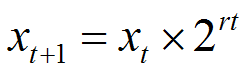
Exponential growth, when describing populations that double periodically (for example, bacteria), can be formulated once three parameters have been defined:
- Total time of growth (mins), typical real-life values of t may range from 0 to 1000;
- Initial population size (symbolised x; where the starting value, x0, is any real, positive integer, consequently x0 must equal or be greater than 1);
- Number of divisions per minute (symbolised r, a useful value for this coefficient for computation is 0.00001).
Hence, the size of the population (x), at time (t) can be calculated from the relationship shown as equation (1) immediately below:
|
equation (1) |
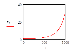
In real situations this mode of population growth cannot continue indefinitely, however. There is usually some limiting factor, such as space or nutrients, that curbs the growth rate (=number of divisions per minute, r).
Monod (1949) was the first to consider this in his mathematical descriptions of bacterial growth. He assumed that it was limitation of nutrients and not cell death that ended the exponential phase of growth, and that growth is proportional to the concentration of the nutrient when looking at individual cells.
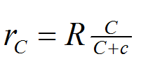
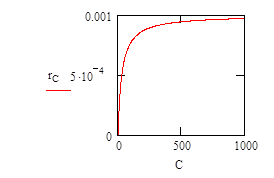
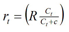
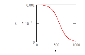
To model this it is necessary to evaluate how the growth rate varies with respect to the concentration of limiting nutient. This is determined experimentally and results in a plot like that (shown below) described by equation (2).
In equation (2), the maximum rate of growth, R, in an unlimited concentration of nutrient is determined (this will be done experimentally, for the sake of the plot shown below for equation (2) this parameter has been given a value of 0.001.
The concentration of nutrient in the system, C, varies between zero and 1000 units; and c is the concentration at which r = rmax/2.
Hence, the relationship can be described with a hyperbolic equation shown below as equation (2).
|
equation (2) |
In order to link these two descriptions, we need to define how the concentration of the limiting nutrient varies with respect to time. This is not a simple matter as the concentration of the nutrient is dependent on the number of individuals in the system which is dependent on the rate of growth of each individual which is dependent on the concentration of the nutrient.
Therefore, it is necessary to approximate the rate of decrease of nutrient concentration independently of the number of individuals consuming it. For this approximation we can assume that the concentration of the nutrient decreases in an exponential way.
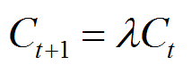
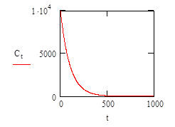
If we define the initial concentration of the nutient, C0 to be 10000 units; and the rate at which it is consumed (λ) = 0.99, then the exponential decease in concentration can be calculated using equation (3):
|
equation (3) |
Then, equation (2) can be re-written with respect to t to illustrate the effect of exponentially diminishing nutrient concentration on the value of r (number of divisions per minute = growth rate), becoming equation (4):
|
equation (4) |
And finally equation (1) can be re-written so that the growth rate varies with time in accord with the diminishing nutrient, and becoming equation (5):
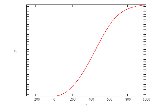
Note that thevertical (y) axis is a logarithmic scale |
equation (5) |
The curve generated by equation (5) describes the population growing initially at an increasing exponential rate (= the lag phase of a real growth curve), then reaching a steady state of exponential increase (= exponential phase), and finally slowing as the concentration of nutrient becomes limiting (deceleration phase).
This is the classic sigmoidal growth curve observed so often in growth experiments with all sorts of organisms and resulting from all sorts of experimental measurement procedures.
While Monod developed these descriptions for bacterial growth, they can be equally well applied to biomass evolution in fungal mycelia. The model of hyphal branching and biomass evolution developed by Prosser & Trinci (1979) is based on the mathematics outlined above.
The most important additional concept emerging from the application of this algebra to the extension growth of filamentous fungi is that in filamentous fungi the increase in number of hyphal branches is equivalent to the increase in number of bacterial cells in a suspension culture of single-celled bacteria. |